
Multitaper F-test for harmonic components
The Slepian sequences of the multitaper spectral estimation method can also be used to perform a hypothesis test regarding the presence of a pure sinusoid at any analyzed frequency. The F-test is used to assess whether the power at a given frequency can be attributed to a single line component. In this case, the power would be given by the summed spectral convolutions of the Slepian frequency functions with the line power spectrum, which is a dirac delta. The complex Fourier coefficient of the putative sinusoid is estimated through a linear regression of the Slepian DC components, and the strength of the regression coefficient is tested against the residual spectral power for the F-test.
The following demonstrates the use of the harmonic test.
import numpy as np
import nitime.algorithms as nt_alg
import nitime.utils as nt_ut
import matplotlib.pyplot as pp
We will set up a test signal with 3 harmonic components within Gaussian noise. The line components must be sufficiently resolved given the multitaper bandwidth of 2NW.
N = 10000
fft_pow = int( np.ceil(np.log2(N) + 2) )
NW = 4
lines = np.sort(np.random.randint(100, 2**(fft_pow-6), size=(3,)))
while np.any( np.diff(lines) < 2*NW ):
    lines = np.sort(np.random.randint(2**(fft_pow-6), size=(3,)))
lines = lines.astype('d')
The harmonic test should find exact frequencies if they were to fall on the FFT grid. (Try commenting the following to see.) In the scenario of real sampled data, increasing the number of FFT points can help to locate the line components.
lines += np.random.randn(3) # displace from grid locations
Now proceed to specify the frequencies, phases, and amplitudes.
lines /= 2.0**(fft_pow-2) # ensure they are well separated

phs = np.random.rand(3) * 2 * np.pi
amps = np.sqrt(2)/2 + np.abs( np.random.randn(3) )
Set the RMS noise power here. Strategies to detect harmonics in low SNR include improving the reliability of the spectral estimate (increasing NW) and/or increasing the number of FFT points. Note that the former option will limit the ability to resolve lines at nearby frequencies.
nz_sig = 1

tx = np.arange(N)
harmonics = amps[:,None]*np.cos( 2*np.pi*tx*lines[:,None] + phs[:,None] )
harmonic = np.sum(harmonics, axis=0)
nz = np.random.randn(N) * nz_sig
sig = harmonic + nz
Take a look at our mock signal.
pp.figure()
pp.subplot(211)
pp.plot(harmonics.T)
pp.xlim(*(np.array([0.2, 0.3])*N).astype('i'))
pp.title('Sinusoid components')
pp.subplot(212)
pp.plot(harmonic, color='k', linewidth=3)
pp.plot(sig, color=(.6, .6, .6), linewidth=2, linestyle='--')
#pp.xlim(2000, 3000)
pp.xlim(*(np.array([0.2, 0.3])*N).astype('i'))
pp.title('Signal in noise')
pp.gcf().tight_layout()

Here we’ll use the utils.detect_lines() function with the given
Slepian properties (NW), and we’ll ensure that we limit spectral bias
by choosing Slepians with concentration factors greater than 0.9. The
arrays returned include the detected line frequencies (f) and their
complex coefficients (b). The frequencies are normalized from \((0,\frac{1}{2})\)
f, b = nt_ut.detect_lines(sig, (NW, 2*NW), low_bias=True, NFFT=2**fft_pow)
h_est = 2*(b[:,None]*np.exp(2j*np.pi*tx*f[:,None])).real

pp.figure()
pp.subplot(211)
pp.plot(harmonics.T, 'c', linewidth=3)
pp.plot(h_est.T, 'r--', linewidth=2)
pp.title('%d lines detected' % h_est.shape[0])
pp.xlim(*(np.array([0.2, 0.3])*N).astype('i'))
pp.subplot(212)
err = harmonic - np.sum(h_est, axis=0)
pp.plot(err**2)
pp.title('Error signal')
pp.show()
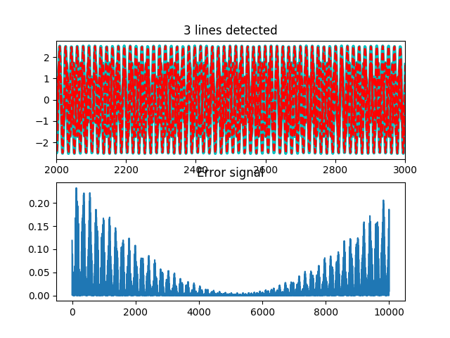
We can see the quality (or not) of our estimated lines. A breakdown of the errors in the various estimated quantities follows in the demo.
phs_est = np.angle(b)
phs_est[phs_est < 0] += 2*np.pi

phs_err = np.linalg.norm(phs_est - phs)**2
amp_err = np.linalg.norm(amps - 2*np.abs(b))**2 / np.linalg.norm(amps)**2
freq_err = np.linalg.norm(lines - f)**2

print('freqs:', lines, '\testimated:', f, '\terr: %1.3e' % freq_err)
print('amp:', amps, '\testimated:', 2*np.abs(b), '\terr: %1.3e' % amp_err)
print('phase:', phs, '\testimated:', phs_est, '\terr: %1.3e' % phs_err)
print('MS error over noise: %1.3e' % (np.mean(err**2)/nz_sig**2,))
Example source code
You can download the full source code of this example.
This same script is also included in the Nitime source distribution under the
doc/examples/ directory.