Fitting an AR model: algorithm module interface

Auto-regressive (AR) processes are processes that follow the following equation:

\[x_t = \sum_{i=1}^{n}a_i * x_{t-i} + \epsilon_t\]

In this example, we will demonstrate the estimation of the AR model coefficients and the estimation of the AR process spectrum, based on the estimation of the coefficients.

We start with imports from numpy, matplotlib and import nitime.utils as well as nitime.algorithms:

import numpy as np
from matplotlib import pyplot as plt

from nitime import utils
from nitime import algorithms as alg
from nitime.timeseries import TimeSeries
from nitime.viz import plot_tseries

We define some variables, which will be used in generating the AR process:

npts = 2048
sigma = 0.1
drop_transients = 128
Fs = 1000

In this case, we generate an order 2 AR process, with the following coefficients:

coefs = np.array([0.9, -0.5])

This generates the AR(2) time series:

X, noise, _ = utils.ar_generator(npts, sigma, coefs, drop_transients)

ts_x = TimeSeries(X, sampling_rate=Fs, time_unit='s')
ts_noise = TimeSeries(noise, sampling_rate=1000, time_unit='s')

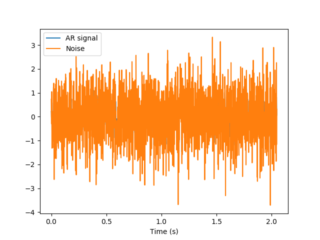
We use the plot_tseries function in order to visualize the process:

fig01 = plot_tseries(ts_x, label='AR signal')
fig01 = plot_tseries(ts_noise, fig=fig01, label='Noise')
fig01.axes[0].legend()

Now we estimate back the model parameters, using two different estimation algorithms.

coefs_est, sigma_est = alg.AR_est_YW(X, 2)
# no rigorous purpose behind 100 transients
X_hat, _, _ = utils.ar_generator(
    N=npts, sigma=sigma_est, coefs=coefs_est, drop_transients=100, v=noise
    )
fig02 = plt.figure()
ax = fig02.add_subplot(111)
ax.plot(np.arange(100, len(X_hat) + 100), X_hat, label='estimated process')
ax.plot(X, 'g--', label='original process')
ax.legend()
err = X_hat - X[100:]
mse = np.dot(err, err) / len(X_hat)
ax.set_title('Mean Square Error: %1.3e' % mse)


plt.show()

Example source code

You can download the full source code of this example. This same script is also included in the Nitime source distribution under the doc/examples/ directory.