Auditory processing in grasshoppers

Extracting the average time-series from one signal, time-locked to the occurrence of some type of event in another signal is a very typical operation in the analysis of time-series from neuroscience experiments. Therefore, we have an additional example of this kind of analysis in Event-related fMRI

In the following code-snippet, we demonstrate the calculation of the spike-triggered average (STA). This is the average of the stimulus wave-form preceding the emission of a spike in the neuron and can be thought of as the stimulus ‘preferred’ by this neuron.

We start by importing the required modules:

import os

import numpy as np

import nitime
import nitime.timeseries as ts
import nitime.analysis as tsa
import nitime.viz as viz
from matplotlib import pyplot as plt

Two data files are used in this example. The first contains the times of action potentials (‘spikes’), recorded intra-cellularly from primary auditory receptors in the grasshopper Locusta Migratoria.

We read in these times and initialize an Events object from them. The spike-times are given in micro-seconds:

data_path = os.path.join(nitime.__path__[0], 'data')

spike_times = np.loadtxt(os.path.join(data_path, 'grasshopper_spike_times1.txt'))

spike_ev = ts.Events(spike_times, time_unit='us')

The first data file contains the stimulus that was played during the recording. Briefly, the stimulus played was a pure-tone in the cell’s preferred frequency amplitude modulated by Gaussian white-noise, up to a cut-off frequency (200 Hz in this case, for details on the experimental procedures and the stimulus see [Rokem2006]).

stim = np.loadtxt(os.path.join(data_path, 'grasshopper_stimulus1.txt'))

The stimulus needs to be transformed from Volts to dB:

def volt2dB(stim, maxdB=100):
    stim = (20 * 1 / np.log(10)) * (np.log(stim[:, 1] / 2.0e-5))
    return maxdB - stim.max() + stim

stim = volt2dB(stim, maxdB=76.4286)  # maxdB taken from the spike file header

We create a time-series object for the stimulus, which was sampled at 20 kHz:

stim_time_series = ts.TimeSeries(t0=0,
                                 data=stim,
                                 sampling_interval=50,
                                 time_unit='us')

Note that the time-representation will not change if we now convert the time-unit into ms. The only thing this accomplishes is to use this time-unit in subsequent visualization of the resulting time-series

stim_time_series.time_unit = 'ms'

Next, we initialize an EventRelatedAnalyzer:

event_related = tsa.EventRelatedAnalyzer(stim_time_series,
                                         spike_ev,
                                         len_et=200,
                                         offset=-200)

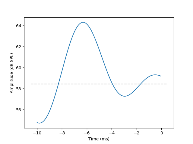
The actual STA gets calculated in this line (the call to ‘event_related.eta’) and the result gets input directly into the plotting function:

fig01 = viz.plot_tseries(event_related.eta, ylabel='Amplitude (dB SPL)')

We prettify the plot a bit by adding a dashed line at the mean of the stimulus

ax = fig01.get_axes()[0]
xlim = ax.get_xlim()
ylim = ax.get_ylim()
mean_stim = np.mean(stim_time_series.data)
ax.plot([xlim[0], xlim[1]], [mean_stim, mean_stim], 'k--')

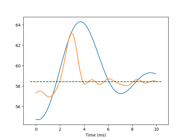
In the following example, a second channel has been added to both the stimulus and the spike-train time-series. This is the response of the same cell, to a different stimulus, in which the frequency modulation has a higher frequency cut-off (800 Hz).

stim2 = np.loadtxt(os.path.join(data_path, 'grasshopper_stimulus2.txt'))
stim2 = volt2dB(stim2, maxdB=76.4286)
spike_times2 = np.loadtxt(os.path.join(data_path, 'grasshopper_spike_times2.txt'))

We loop over the two spike-time events and stimulus time-series:

et = []
means = []
for stim, spike in zip([stim, stim2], [spike_times, spike_times2]):
    stim_time_series = ts.TimeSeries(t0=0, data=stim, sampling_interval=50,
                                     time_unit='us')

    stim_time_series.time_unit = 'ms'

    spike_ev = ts.Events(spike, time_unit='us')
    #Initialize the event-related analyzer
    event_related = tsa.EventRelatedAnalyzer(stim_time_series,
                                             spike_ev,
                                             len_et=200,
                                             offset=-200)

This is the line which actually executes the analysis

et.append(event_related.eta)
means.append(np.mean(stim_time_series.data))

Stack the data from both time-series, initialize a new time-series and plot it:

fig02 = viz.plot_tseries(
    ts.TimeSeries(data=np.vstack([et[0].data, et[1].data]),
                  sampling_rate=et[0].sampling_rate, time_unit='ms'))

ax = fig02.get_axes()[0]
xlim = ax.get_xlim()
ax.plot([xlim[0], xlim[1]], [means[0], means[0]], 'b--')
ax.plot([xlim[0], xlim[1]], [means[1], means[1]], 'g--')

plt.show() is called in order to display the figures

plt.show()

The data used in this example is also available on the CRCNS data sharing web-site.

[Rokem2006]

Ariel Rokem, Sebastian Watzl, Tim Gollisch, Martin Stemmler, Andreas V M Herz and Ines Samengo (2006). Spike-timing precision underlies the coding efficiency of auditory receptor neurons. J Neurophysiol, 95:2541–52

Example source code

You can download the full source code of this example. This same script is also included in the Nitime source distribution under the doc/examples/ directory.