
Multitaper method for baseband demodulation
Another application of the Slepian functions is to estimate the complex demodulate of a narrowband signal. This signal is normally of interest in neuroimaging when finding the lowpass power envelope and the instantaneous phase. The traditional technique uses the Hilbert transform to find the analytic signal. However, this approach suffers problems of bias and reliability, much like the periodogram suffers in PSD estimation. Once again, a multitaper approach can provide an estimate with lower variance.
The following demonstrates the use of spectra of multiple windows to compute a power envelope of a signal in a desired band.
import numpy as np
import scipy.signal as signal
import nitime.algorithms as nt_alg
import nitime.utils as nt_ut
import matplotlib.pyplot as pp
We’ll set up a test signal with a red spectrum (integrated Gaussian noise).
N = 10000
nfft = np.power( 2, int(np.ceil(np.log2(N))) )
NW = 40
W = float(NW)/N
Create a nearly lowpass band-limited signal.
s = np.cumsum( np.random.randn(N) )
Strictly enforce the band-limited property in this signal.
(b, a) = signal.butter(3, W, btype='lowpass')
slp = signal.lfilter(b, a, s)
Modulate both signals away from baseband.
s_mod = s * np.cos(2*np.pi*np.arange(N) * float(200) / N)
slp_mod = slp * np.cos(2*np.pi*np.arange(N) * float(200) / N)
fm = int( np.round(float(200) * nfft / N) )
Create Slepians with the desired bandpass resolution (2W).
(dpss, eigs) = nt_alg.dpss_windows(N, NW, 2*NW)
keep = eigs > 0.9
dpss = dpss[keep]; eigs = eigs[keep]
Test 1
We’ll compare multitaper baseband power estimation with regular Hilbert transform method under actual narrowband conditions.
# MT method
xk = nt_alg.tapered_spectra(slp_mod, dpss, NFFT=nfft)
mtm_bband = np.sum( 2 * (xk[:,fm] * np.sqrt(eigs))[:,None] * dpss, axis=0 )

# Hilbert transform method
hb_bband = signal.hilbert(slp_mod, N=nfft)[:N]

pp.figure()
pp.subplot(211)
pp.plot(slp_mod, 'g')
pp.plot(np.abs(mtm_bband), color='b', linewidth=3)
pp.title('Multitaper Baseband Power')

pp.subplot(212)
pp.plot(slp_mod, 'g')
pp.plot(np.abs(hb_bband), color='b', linewidth=3)
pp.title('Hilbert Baseband Power')
pp.gcf().tight_layout()
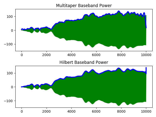
We see in the narrowband signal case that there’s not much difference between taking the Hilbert transform and calculating the multitaper complex demodulate.
Test 2
Now we’ll compare multitaper baseband power estimation with regular Hilbert transform method under more realistic non-narrowband conditions.
# MT method
xk = nt_alg.tapered_spectra(s_mod, dpss, NFFT=nfft)
w, n = nt_ut.adaptive_weights(xk, eigs, sides='onesided')
mtm_bband = np.sum( 2 * (xk[:,fm] * np.sqrt(eigs))[:,None] * dpss, axis=0 )

# Hilbert transform method
hb_bband = signal.hilbert(s_mod, N=nfft)[:N]

pp.figure()
pp.subplot(211)
pp.plot(s_mod, 'g')
pp.plot(np.abs(mtm_bband), color='b', linewidth=3)
pp.title('Multitaper Baseband Power')

pp.subplot(212)
pp.plot(s_mod, 'g')
pp.plot(np.abs(hb_bband), color='b', linewidth=3)
pp.title('Hilbert Baseband Power')
pp.gcf().tight_layout()
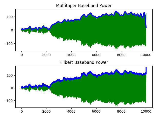
Here we see that since the underlying signal is not truly narrowband, the broadband bias is corrupting the Hilbert transform estimation of the complex demodulate. However the multitaper estimate clearly remains lowpass.
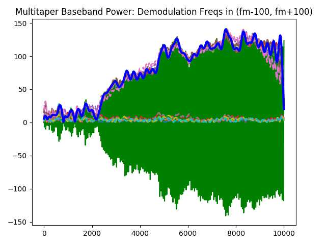
Another property of computing the complex demodulate from the spectra of multiple windows is that all bandpasses can be computed. In the above examples, we were only taking a slice from the modulation frequency that we set up. In practice, we might be interested in bandpasses at various frequencies. Note here, though, that our bandwidth is set by the Slepian sequences we used for analysis. The following plot shows a family of complex demodulates at frequencies near the modulation frequency.
### Show a family of baseband demodulations from the multitaper method
#eigen_coefs = 2 * (xk[:,(fm-100):(fm+100):10] * np.sqrt(eigs)[:,None])
eigen_coefs = 2 * (xk[:,(fm-100):(fm+100):10] * \
                   np.sqrt(w[:,(fm-100):(fm+100):10]))
mtm_fbband = np.sum( eigen_coefs[:,:,None] * dpss[:,None,:], axis=0 )

pp.figure()
pp.plot(s_mod, 'g')
pp.plot(np.abs(mtm_fbband).T, linestyle='--', linewidth=2)
pp.plot(np.abs(mtm_bband), color='b', linewidth=3)
pp.title('Multitaper Baseband Power: Demodulation Freqs in (fm-100, fm+100)')
pp.gcf().tight_layout()
pp.show()
Example source code
You can download the full source code of this example.
This same script is also included in the Nitime source distribution under the
doc/examples/ directory.