Filtering and normalizing fMRI data

Filtering fMRI data is very important. The time-series usually collected in fMRI contain a broad-band signal. However, physilogically relevant signals are thought to be present in only particular parts of the spectrum. For this reason, filtering operations, such as detrending, are a common pre-processing step in analysis of fMRI data analysis. In addition, for many fMRI analyses, it is important to normalize the data in each voxel. This is because data may differ between different voxels for ‘uninteresting’ reasons, such as local blood-flow differences and signal amplitude differences due to the distance from the receive coil. In the following, we will demonstrate usage of nitimes analyzer objects for spectral estimation, filtering and normalization on fMRI data.

We start by importing the needed modules. First modules from the standard lib and from 3rd parties:

import os

import numpy as np
import matplotlib.pyplot as plt

Next, the particular nitime classes we will be using in this example:

import nitime

# Import the time-series objects:
from nitime.timeseries import TimeSeries

# Import the analysis objects:
from nitime.analysis import SpectralAnalyzer, FilterAnalyzer, NormalizationAnalyzer

For starters, let’s analyze data that has been preprocessed and is extracted into indivudal ROIs. This is the same data used in Multitaper coherence estimation and in Coherency analysis of fMRI data (see these examples for details).

We start by setting the TR and reading the data from the CSV table into which the data was saved:

TR = 1.89

data_path = os.path.join(nitime.__path__[0], 'data')

data = np.loadtxt(os.path.join(data_path, 'fmri_timeseries.csv'),
                  skiprows=1, delimiter=',')

# Extract ROI information from the csv file headers:
roi_names = np.array(data_rec.dtype.names)

# This is the number of samples in each ROI:
n_samples = data_rec.shape[0]

# Make an empty container for the data
data = np.zeros((len(roi_names), n_samples))

# Insert the data from each ROI into a row in the data:
for n_idx, roi in enumerate(roi_names):
    data[n_idx] = data_rec[roi]

# Initialize TimeSeries object:
T = TimeSeries(data, sampling_interval=TR)
T.metadata['roi'] = roi_names

We will start, by examining the spectrum of the original data, before filtering. We do this by initializing a SpectralAnalyzer for the original data:

S_original = SpectralAnalyzer(T)

# Initialize a figure to put the results into:
fig01 = plt.figure()
ax01 = fig01.add_subplot(1, 1, 1)

The spectral analyzer has several different methods of spectral analysis, however the all have a common API. This means that for all of them the output is a tuple. The first item in the tuple are the central frequencies of the frequency bins in the spectrum and the second item in the tuple are the magnitude of the spectrum in that frequency bin. For the purpose of this example, we will only plot the data from the 10th ROI (by indexing into the spectra). We compare all the methods of spectral estimation by plotting them together:

ax01.plot(S_original.psd[0],
          S_original.psd[1][9],
          label='Welch PSD')

ax01.plot(S_original.spectrum_fourier[0],
          np.abs(S_original.spectrum_fourier[1][9]),
          label='FFT')

ax01.plot(S_original.periodogram[0],
          S_original.periodogram[1][9],
          label='Periodogram')

ax01.plot(S_original.spectrum_multi_taper[0],
          S_original.spectrum_multi_taper[1][9],
          label='Multi-taper')

ax01.set_xlabel('Frequency (Hz)')
ax01.set_ylabel('Power')

ax01.legend()

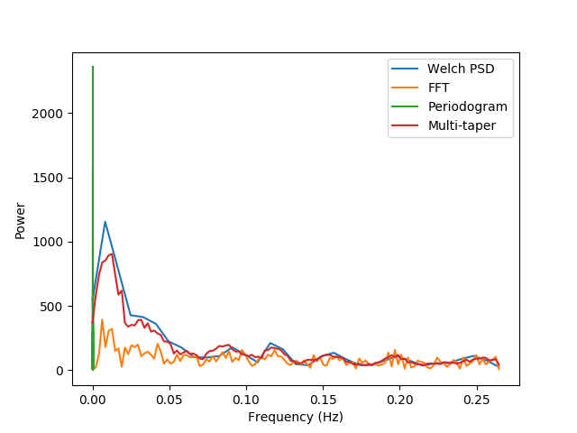
Notice that, for this data, simply extracting a FFT is hardly informative (the reasons for that are explained in Multitaper spectral estimation). On the other hand, the other methods provide different granularity of information, traded-off with the robustness of the estimation. The cadillac of spectral estimates is the multi-taper estimation, which provides both robustness and granularity, but notice that this estimate requires more computation than other estimates (certainly more estimates than the FFT).

We note that a lot of the power in the fMRI data seems to be concentrated in frequencies below 0.02 Hz. These extremely low fluctuations in signal are often considered to be ‘noise’, rather than reflecting neural processing. In addition, there is a broad distribution of power up to the Nyquist frequency. However, some estimates of the hemodynamic response suggest that information above 0.15 could not reflect the slow filtering of neural response to the BOLD response measured in fMRI. Thus, it would be advantageous to remove fluctuations below 0.02 and above 0.15 Hz from the data. Next, we proceed to filter the data into this range, using different methods.

We start by initializing a FilterAnalyzer. This is initialized with the time-series containing the data and with the upper and lower bounds of the range into which we wish to filter (in Hz):

F = FilterAnalyzer(T, ub=0.15, lb=0.02)

# Initialize a figure to display the results:
fig02 = plt.figure()
ax02 = fig02.add_subplot(1, 1, 1)

# Plot the original, unfiltered data:
ax02.plot(F.data[0], label='unfiltered')

As with the SpectralAnalyzer, there is a common API for the different methods used for filtering. We use the following methods:

• Boxcar filter: The time-series is convolved with a box-car function of the right length to smooth the data to such an extent that the frequencies higher than represented by the length of this box-car function are no longer present in the smoothed version of the time-series. This functions as a low-pass filter. The data can then be high-pass filtered by subtracting this version of the data from the original. For a band-pass filter, both of these operations are done.

ax02.plot(F.filtered_boxcar.data[0], label='Boxcar filter')

• FIR filter: A digital filter with a finite impulse response. These filters have an order of 64 per default, but that can be adjusted by setting the key word argument ‘filt_order’, passed to initialize the FilterAnalyzer. For FIR filtering, nitime uses a Hamming window filter, but this can also be changed by setting the key word argument ‘fir_win’. As with the boxcar filter, if band-pass filtering is required, a low-pass filter is applied and then a high-pass filter is applied to the resulting time-series.

ax02.plot(F.fir.data[0], label='FIR')

• IIR filter: A digital filter with an infinite impulse response function. Per default an elliptic filter is used here, but this can be changed, by setting the ‘iir_type’ key word argument used when initializing the FilterAnalyzer.

For both FIR filters and IIR filters, scipy.signal.filtfilt() is used in order to achieve zero phase delay filtering.

ax02.plot(F.iir.data[0], label='IIR')

• Fourier filter: this is a quick and dirty filter. The data is FFT-ed into the frequency domain. The power in the unwanted frequency bins is removed (by replacing the power in these bins with zero) and the data is IFFT-ed back into the time-domain.

ax02.plot(F.filtered_fourier.data[0], label='Fourier')
ax02.legend()
ax02.set_xlabel('Time (TR)')
ax02.set_ylabel('Signal amplitude (a.u.)')

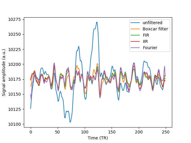
Examining the resulting time-series closely reveals that large fluctuations in very slow frequencies have been removed, but also small fluctuations in high frequencies have been attenuated through filtering.

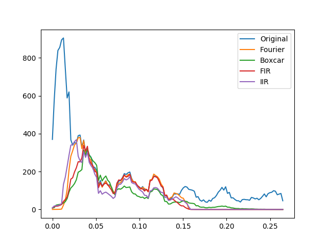
Comparing the resulting spectra of these different filters shows the various trade-offs of each filtering method, including the fidelity with which the original spectrum is replicated within the pass-band and the amount of attenuation within the stop-bands.

We can do that by initializng a SpectralAnalyzer for each one of the filtered time-series resulting from the above operation and plotting their spectra. For ease of compariso, we only plot the spectra using the multi-taper spectral estimation. At the level of granularity provided by this method, the diferences between the methods are emphasized:

S_fourier = SpectralAnalyzer(F.filtered_fourier)
S_boxcar = SpectralAnalyzer(F.filtered_boxcar)
S_fir = SpectralAnalyzer(F.fir)
S_iir = SpectralAnalyzer(F.iir)

fig03 = plt.figure()
ax03 = fig03.add_subplot(1, 1, 1)

ax03.plot(S_original.spectrum_multi_taper[0],
          S_original.spectrum_multi_taper[1][9],
          label='Original')

ax03.plot(S_fourier.spectrum_multi_taper[0],
          S_fourier.spectrum_multi_taper[1][9],
          label='Fourier')

ax03.plot(S_boxcar.spectrum_multi_taper[0],
          S_boxcar.spectrum_multi_taper[1][9],
          label='Boxcar')

ax03.plot(S_fir.spectrum_multi_taper[0],
          S_fir.spectrum_multi_taper[1][9],
          label='FIR')

ax03.plot(S_iir.spectrum_multi_taper[0],
          S_iir.spectrum_multi_taper[1][9],
          label='IIR')

ax03.legend()

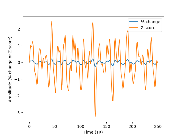
Next, we turn to normalize the filtered data. This can be done in one of two methods:

• Percent change: the data in each voxel is normalized as percent signal change, relative to the mean BOLD signal in the voxel
• Z score: The data in each voxel is normalized to have 0 mean and a standard deviation of 1.

We will use the filtered data, in order to demonstrate how the output of one analyzer can be used as the input to the other:

fig04 = plt.figure()
ax04 = fig04.add_subplot(1, 1, 1)

ax04.plot(NormalizationAnalyzer(F.fir).percent_change.data[0], label='% change')
ax04.plot(NormalizationAnalyzer(F.fir).z_score.data[0], label='Z score')
ax04.legend()
ax04.set_xlabel('Time (TR)')
ax04.set_ylabel('Amplitude (% change or Z-score)')

Notice that the same methods of filtering and normalization can be applied to fMRI data, upon reading it from a nifti file, using nitime.fmri.io.

We demonstrate that in what follows.[Notice that nibabel (http://nipy.org/nibabel) is required in order to run the following examples. An error will be thrown if nibabel is not installed]

try:
    from nibabel import load
except ImportError:
    raise ImportError('You need nibabel (http:/nipy.org/nibabel/) in order to run this example')

import nitime.fmri.io as io

We define the TR of the analysis and the frequency band of interest:

TR = 1.35
f_lb = 0.02
f_ub = 0.15

An fMRI data file with some fMRI data is shipped as part of the distribution, the following line will find the path to this data on the specific computer:

data_file_path = test_dir_path = os.path.join(nitime.__path__[0],
                                              'data')

fmri_file = os.path.join(data_file_path, 'fmri1.nii.gz')

Read in the dimensions of the data, using nibabel:

fmri_data = load(fmri_file)
volume_shape = fmri_data.shape[:-1]
coords = list(np.ndindex(volume_shape))
coords = np.array(coords).T

We use nitime.fmri.io in order to generate a TimeSeries object from spatial coordinates in the data file. Notice that normalization method is provided as a string input to the keyword argument ‘normalize’ and the filter and its properties are provided as a dict to the keyword argument ‘filter’:

T_unfiltered = io.time_series_from_file(fmri_file,
                                        coords,
                                        TR=TR,
                                        normalize='percent')

T_fir = io.time_series_from_file(fmri_file,
                              coords,
                              TR=TR,
                              normalize='percent',
                              filter=dict(lb=f_lb,
                                          ub=f_ub,
                                          method='fir',
                                          filt_order=10))

T_iir = io.time_series_from_file(fmri_file,
                              coords,
                              TR=TR,
                              normalize='percent',
                              filter=dict(lb=f_lb,
                                          ub=f_ub,
                                          method='iir',
                                          filt_order=10))

T_boxcar = io.time_series_from_file(fmri_file,
                              coords,
                              TR=TR,
                              normalize='percent',
                              filter=dict(lb=f_lb,
                                          ub=f_ub,
                                          method='boxcar',
                                          filt_order=10))

fig05 = plt.figure()
ax05 = fig05.add_subplot(1, 1, 1)
S_unfiltered = SpectralAnalyzer(T_unfiltered).spectrum_multi_taper
S_fir = SpectralAnalyzer(T_fir).spectrum_multi_taper
S_iir = SpectralAnalyzer(T_iir).spectrum_multi_taper
S_boxcar = SpectralAnalyzer(T_boxcar).spectrum_multi_taper

random_voxel = np.random.randint(0, np.prod(volume_shape))

ax05.plot(S_unfiltered[0], S_unfiltered[1][random_voxel], label='Unfiltered')
ax05.plot(S_fir[0], S_fir[1][random_voxel], label='FIR filtered')
ax05.plot(S_iir[0], S_iir[1][random_voxel], label='IIR filtered')
ax05.plot(S_boxcar[0], S_boxcar[1][random_voxel], label='Boxcar filtered')
ax05.legend()

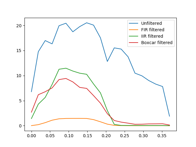
Notice that though the boxcar filter doesn’t usually do an amazing job with long time-series and IIR/FIR filters seem to be superior in those cases, in this example, where the time-series is much shorter, it sometimes does a relatively decent job.

We call plt.show() in order to display the figure:

plt.show()

Example source code

You can download the full source code of this example. This same script is also included in the Nitime source distribution under the doc/examples/ directory.