
Multitaper coherence estimation
Coherence estimation can be done using windowed-spectra. This is the method used in the example Coherency analysis of fMRI data. In addition, multitaper spectral estimation can be used in order to calculate coherence and also confidence intervals for the coherence values that result (see Multitaper spectral estimation)
The data analyzed here is an fMRI data-set contributed by Beth Mormino. The data is taken from a single subject in a “resting-state” scan, in which subjects are fixating on a cross and maintaining alert wakefulness, but not performing any other behavioral task.
We start by importing modules/functions we will use in this example and define variables which will be used as the sampling interval of the TimeSeries objects and as upper and lower bounds on the frequency range analyzed:
import os

import numpy as np
import matplotlib.pyplot as plt
import scipy.stats.distributions as dist
from scipy import fftpack

import nitime
from nitime.timeseries import TimeSeries
from nitime import utils
import nitime.algorithms as alg
import nitime.viz
from nitime.viz import drawmatrix_channels
from nitime.analysis import CoherenceAnalyzer, MTCoherenceAnalyzer

TR = 1.89
f_ub = 0.15
f_lb = 0.02
We read in the data into a recarray from a csv file:
data_path = os.path.join(nitime.__path__[0], 'data')

fname = os.path.join(data_path, 'fmri_timeseries.csv')

data_rec = np.genfromtxt(fname, dtype=float, delimiter=',', names=True)
The first line in the file contains the names of the different brain regions (or ROI = regions of interest) from which the time-series were derived. We extract the data into a regular array, while keeping the names to be used later:
roi_names = np.array(data_rec.dtype.names)
nseq = len(roi_names)
n_samples = data_rec.shape[0]
data = np.zeros((nseq, n_samples))

for n_idx, roi in enumerate(roi_names):
    data[n_idx] = data_rec[roi]
We normalize the data in each of the ROIs to be in units of % change:
pdata = utils.percent_change(data)
We start by performing the detailed analysis, but note that a significant short-cut is presented below, so if you just want to know how to do this (without needing to understand the details), skip on down.
We start by defining how many tapers will be used and calculate the values of the tapers and the associated eigenvalues of each taper:
NW = 4
K = 2 * NW - 1

tapers, eigs = alg.dpss_windows(n_samples, NW, K)
We multiply the data by the tapers and derive the Fourier transform and the magnitude of the squared spectra (the power) for each tapered time-series:
tdata = tapers[None, :, :] * pdata[:, None, :]
tspectra = fftpack.fft(tdata)
## mag_sqr_spectra = np.abs(tspectra)
## np.power(mag_sqr_spectra, 2, mag_sqr_spectra)
Coherence for real sequences is symmetric, so we calculate this for only half the spectrum (the other half is equal):
L = n_samples // 2 + 1
sides = 'onesided'
We estimate adaptive weighting of the tapers, based on the data (see Multitaper spectral estimation for an explanation and references):
w = np.empty((nseq, K, L))
for i in range(nseq):
    w[i], _ = utils.adaptive_weights(tspectra[i], eigs, sides=sides)
We proceed to calculate the coherence. We initialize empty data containers:
csd_mat = np.zeros((nseq, nseq, L), 'D')
psd_mat = np.zeros((2, nseq, nseq, L), 'd')
coh_mat = np.zeros((nseq, nseq, L), 'd')
coh_var = np.zeros_like(coh_mat)
Looping over the ROIs:
for i in range(nseq):
    for j in range(i):
We calculate the multi-tapered cross spectrum between each two time-series:
sxy = alg.mtm_cross_spectrum(
   tspectra[i], tspectra[j], (w[i], w[j]), sides='onesided'
 )
And the individual PSD for each:
sxx = alg.mtm_cross_spectrum(
   tspectra[i], tspectra[i], w[i], sides='onesided'
   )
syy = alg.mtm_cross_spectrum(
   tspectra[j], tspectra[j], w[j], sides='onesided'
   )

psd_mat[0, i, j] = sxx
psd_mat[1, i, j] = syy
Coherence is : \(Coh_{xy}(\lambda) = \frac{|{f_{xy}(\lambda)}|^2}{f_{xx}(\lambda) \cdot f_{yy}(\lambda)}\)
coh_mat[i, j] = np.abs(sxy) ** 2
coh_mat[i, j] /= (sxx * syy)
csd_mat[i, j] = sxy
The variance from the different samples is calculated using a jack-knife approach:
if i != j:
    coh_var[i, j] = utils.jackknifed_coh_variance(
       tspectra[i], tspectra[j], eigs, adaptive=True,
       )
This measure is normalized, based on the number of tapers:
coh_mat_xform = utils.normalize_coherence(coh_mat, 2 * K - 2)
We calculate 95% confidence intervals based on the jack-knife variance calculation:
t025_limit = coh_mat_xform + dist.t.ppf(.025, K - 1) * np.sqrt(coh_var)
t975_limit = coh_mat_xform + dist.t.ppf(.975, K - 1) * np.sqrt(coh_var)


utils.normal_coherence_to_unit(t025_limit, 2 * K - 2, t025_limit)
utils.normal_coherence_to_unit(t975_limit, 2 * K - 2, t975_limit)

if L < n_samples:
    freqs = np.linspace(0, 1 / (2 * TR), L)
else:
    freqs = np.linspace(0, 1 / TR, L, endpoint=False)
We look only at frequencies between 0.02 and 0.15 (the physiologically relevant band, see http://imaging.mrc-cbu.cam.ac.uk/imaging/DesignEfficiency:
freq_idx = np.where((freqs > f_lb) * (freqs < f_ub))[0]
We extract the coherence and average over all these frequency bands:
coh = np.mean(coh_mat[:, :, freq_idx], -1) # Averaging on the last dimension
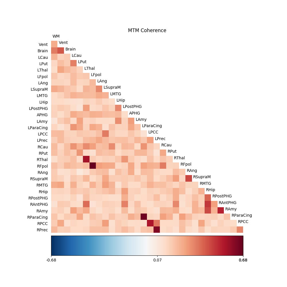
The next line calls the visualization routine which displays the data:
fig01 = drawmatrix_channels(coh,
                            roi_names,
                            size=[10., 10.],
                            color_anchor=0,
                            title='MTM Coherence')
Next we perform the same analysis, using the nitime object oriented interface.
We start by initializing a TimeSeries object with this data and with the sampling_interval provided above. We set the metadata ‘roi’ field with the ROI names.
T = TimeSeries(pdata, sampling_interval=TR)
T.metadata['roi'] = roi_names
We initialize an MTCoherenceAnalyzer object with the TimeSeries object:
C2 = MTCoherenceAnalyzer(T)
The relevant indices in the Analyzer object are derived:
freq_idx = np.where((C2.frequencies > 0.02) * (C2.frequencies < 0.15))[0]
The call to C2.coherence triggers the computation and this is averaged over the frequency range of interest in the same line and then displayed:
coh = np.mean(C2.coherence[:, :, freq_idx], -1)  # Averaging on the last dimension
fig02 = drawmatrix_channels(coh,
                            roi_names,
                            size=[10., 10.],
                            color_anchor=0,
                            title='MTCoherenceAnalyzer')

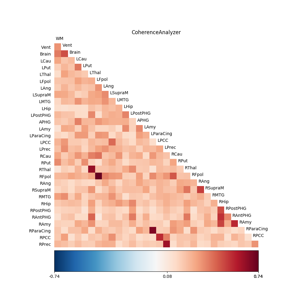
For comparison, we also perform the analysis using the standard CoherenceAnalyzer object, which does the analysis using Welch’s windowed periodogram, instead of the multitaper spectral estimation method (see resting_state for a more thorough analysis of this data using this method):
C3 = CoherenceAnalyzer(T)

freq_idx = np.where((C3.frequencies > f_lb) * (C3.frequencies < f_ub))[0]

#Extract the coherence and average across these frequency bands:
coh = np.mean(C3.coherence[:, :, freq_idx], -1)  # Averaging on the last dimension
fig03 = drawmatrix_channels(coh,
                            roi_names,
                            size=[10., 10.],
                            color_anchor=0,
                            title='CoherenceAnalyzer')
plt.show() is called in order to display the figures:
plt.show()
Example source code
You can download the full source code of this example.
This same script is also included in the Nitime source distribution under the
doc/examples/ directory.