algorithms.statistics.models.regression

Module: algorithms.statistics.models.regression

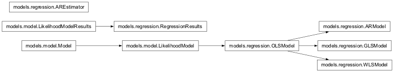
Inheritance diagram for nipy.algorithms.statistics.models.regression:

This module implements some standard regression models: OLS and WLS models, as well as an AR(p) regression model.

Models are specified with a design matrix and are fit using their ‘fit’ method.

Subclasses that have more complicated covariance matrices should write over the ‘whiten’ method as the fit method prewhitens the response by calling ‘whiten’.

General reference for regression models:

‘Introduction to Linear Regression Analysis’, Douglas C. Montgomery,

Elizabeth A. Peck, G. Geoffrey Vining. Wiley, 2006.

Classes

AREstimator

class nipy.algorithms.statistics.models.regression.AREstimator(model, p=1)

Bases: object

A class to estimate AR(p) coefficients from residuals

__init__(model, p=1)

Bias-correcting AR estimation class

Parameters:

modelOSLModel instance

A models.regression.OLSmodel instance, where model has attribute design

pint, optional

Order of AR(p) noise

ARModel

class nipy.algorithms.statistics.models.regression.ARModel(design, rho)

Bases: OLSModel

A regression model with an AR(p) covariance structure.

In terms of a LikelihoodModel, the parameters are beta, the usual regression parameters, and sigma, a scalar nuisance parameter that shows up as multiplier in front of the AR(p) covariance.

The linear autoregressive process of order p–AR(p)–is defined as:

TODO

Examples

>>> from nipy.algorithms.statistics.api import Term, Formula
>>> data = np.rec.fromarrays(([1,3,4,5,8,10,9], range(1,8)),
...                          names=('Y', 'X'))
>>> f = Formula([Term("X"), 1])
>>> dmtx = f.design(data, return_float=True)
>>> model = ARModel(dmtx, 2)

We go through the model.iterative_fit procedure long-hand:

>>> for i in range(6):
...     results = model.fit(data['Y'])
...     print("AR coefficients:", model.rho)
...     rho, sigma = yule_walker(data["Y"] - results.predicted,
...                              order=2,
...                              df=model.df_resid)
...     model = ARModel(model.design, rho) 
...
AR coefficients: [ 0.  0.]
AR coefficients: [-0.61530877 -1.01542645]
AR coefficients: [-0.72660832 -1.06201457]
AR coefficients: [-0.7220361  -1.05365352]
AR coefficients: [-0.72229201 -1.05408193]
AR coefficients: [-0.722278   -1.05405838]
>>> results.theta 
array([ 1.59564228, -0.58562172])
>>> results.t() 
array([ 38.0890515 ,  -3.45429252])
>>> print(results.Tcontrast([0,1]))  
<T contrast: effect=-0.58562172384377043, sd=0.16953449108110835,
t=-3.4542925165805847, df_den=5>
>>> print(results.Fcontrast(np.identity(2)))  
<F contrast: F=4216.810299725842, df_den=5, df_num=2>

Reinitialize the model, and do the automated iterative fit

>>> model.rho = np.array([0,0])
>>> model.iterative_fit(data['Y'], niter=3)
>>> print(model.rho)  
[-0.7220361  -1.05365352]

__init__(design, rho)

Initialize AR model instance

Parameters:

designndarray

2D array with design matrix

rhoint or array-like

If int, gives order of model, and initializes rho to zeros. If ndarray, gives initial estimate of rho. Be careful as ARModel(X, 1) != ARModel(X, 1.0).

fit(Y)

Fit model to data Y

Full fit of the model including estimate of covariance matrix, (whitened) residuals and scale.

Parameters:

Yarray-like

The dependent variable for the Least Squares problem.

Returns:

fitRegressionResults

has_intercept()

Check if column of 1s is in column space of design

information(beta, nuisance=None)

Returns the information matrix at (beta, Y, nuisance).

See logL for details.

Parameters:

betandarray

The parameter estimates. Must be of length df_model.

nuisancedict

A dict with key ‘sigma’, which is an estimate of sigma. If None, defaults to its maximum likelihood estimate (with beta fixed) as sum((Y - X*beta)**2) / n where n=Y.shape[0], X=self.design.

Returns:

infoarray

The information matrix, the negative of the inverse of the Hessian of the of the log-likelihood function evaluated at (theta, Y, nuisance).

initialize(design)

Initialize (possibly re-initialize) a Model instance.

For instance, the design matrix of a linear model may change and some things must be recomputed.

iterative_fit(Y, niter=3)

Perform an iterative two-stage procedure to estimate AR(p) parameters and regression coefficients simultaneously.

Parameters:

Yndarray

data to which to fit model

niteroptional, int

the number of iterations (default 3)

Returns:

None

logL(beta, Y, nuisance=None)

Returns the value of the loglikelihood function at beta.

Given the whitened design matrix, the loglikelihood is evaluated at the parameter vector, beta, for the dependent variable, Y and the nuisance parameter, sigma.

Parameters:

betandarray

The parameter estimates. Must be of length df_model.

Yndarray

The dependent variable

nuisancedict, optional

A dict with key ‘sigma’, which is an optional estimate of sigma. If None, defaults to its maximum likelihood estimate (with beta fixed) as sum((Y - X*beta)**2) / n, where n=Y.shape[0], X=self.design.

Returns:

loglffloat

The value of the loglikelihood function.

Notes

The log-Likelihood Function is defined as

\[\ell(\beta,\sigma,Y)= -\frac{n}{2}\log(2\pi\sigma^2) - \|Y-X\beta\|^2/(2\sigma^2)\]

The parameter \(\sigma\) above is what is sometimes referred to as a nuisance parameter. That is, the likelihood is considered as a function of \(\beta\), but to evaluate it, a value of \(\sigma\) is needed.

If \(\sigma\) is not provided, then its maximum likelihood estimate:

\[\hat{\sigma}(\beta) = \frac{\text{SSE}(\beta)}{n}\]

is plugged in. This likelihood is now a function of only \(\beta\) and is technically referred to as a profile-likelihood.

References

[1]

23. Green. “Econometric Analysis,” 5th ed., Pearson, 2003.

predict(design=None)

After a model has been fit, results are (assumed to be) stored in self.results, which itself should have a predict method.

rank()

Compute rank of design matrix

score(beta, Y, nuisance=None)

Gradient of the loglikelihood function at (beta, Y, nuisance).

The graient of the loglikelihood function at (beta, Y, nuisance) is the score function.

See logL() for details.

Parameters:

betandarray

The parameter estimates. Must be of length df_model.

Yndarray

The dependent variable.

nuisancedict, optional

A dict with key ‘sigma’, which is an optional estimate of sigma. If None, defaults to its maximum likelihood estimate (with beta fixed) as sum((Y - X*beta)**2) / n, where n=Y.shape[0], X=self.design.

Returns:

The gradient of the loglikelihood function.

whiten(X)

Whiten a series of columns according to AR(p) covariance structure

Parameters:

Xarray-like of shape (n_features)

array to whiten

Returns:

wXndarray

X whitened with order self.order AR

GLSModel

class nipy.algorithms.statistics.models.regression.GLSModel(design, sigma)

Bases: OLSModel

Generalized least squares model with a general covariance structure

__init__(design, sigma)

Parameters:

designarray-like

This is your design matrix. Data are assumed to be column ordered with observations in rows.

fit(Y)

Fit model to data Y

Full fit of the model including estimate of covariance matrix, (whitened) residuals and scale.

Parameters:

Yarray-like

The dependent variable for the Least Squares problem.

Returns:

fitRegressionResults

has_intercept()

Check if column of 1s is in column space of design

information(beta, nuisance=None)

Returns the information matrix at (beta, Y, nuisance).

See logL for details.

Parameters:

betandarray

The parameter estimates. Must be of length df_model.

nuisancedict

A dict with key ‘sigma’, which is an estimate of sigma. If None, defaults to its maximum likelihood estimate (with beta fixed) as sum((Y - X*beta)**2) / n where n=Y.shape[0], X=self.design.

Returns:

infoarray

The information matrix, the negative of the inverse of the Hessian of the of the log-likelihood function evaluated at (theta, Y, nuisance).

initialize(design)

Initialize (possibly re-initialize) a Model instance.

For instance, the design matrix of a linear model may change and some things must be recomputed.

logL(beta, Y, nuisance=None)

Returns the value of the loglikelihood function at beta.

Given the whitened design matrix, the loglikelihood is evaluated at the parameter vector, beta, for the dependent variable, Y and the nuisance parameter, sigma.

Parameters:

betandarray

The parameter estimates. Must be of length df_model.

Yndarray

The dependent variable

nuisancedict, optional

A dict with key ‘sigma’, which is an optional estimate of sigma. If None, defaults to its maximum likelihood estimate (with beta fixed) as sum((Y - X*beta)**2) / n, where n=Y.shape[0], X=self.design.

Returns:

loglffloat

The value of the loglikelihood function.

Notes

The log-Likelihood Function is defined as

\[\ell(\beta,\sigma,Y)= -\frac{n}{2}\log(2\pi\sigma^2) - \|Y-X\beta\|^2/(2\sigma^2)\]

The parameter \(\sigma\) above is what is sometimes referred to as a nuisance parameter. That is, the likelihood is considered as a function of \(\beta\), but to evaluate it, a value of \(\sigma\) is needed.

If \(\sigma\) is not provided, then its maximum likelihood estimate:

\[\hat{\sigma}(\beta) = \frac{\text{SSE}(\beta)}{n}\]

is plugged in. This likelihood is now a function of only \(\beta\) and is technically referred to as a profile-likelihood.

References

[1]

23. Green. “Econometric Analysis,” 5th ed., Pearson, 2003.

predict(design=None)

After a model has been fit, results are (assumed to be) stored in self.results, which itself should have a predict method.

rank()

Compute rank of design matrix

score(beta, Y, nuisance=None)

Gradient of the loglikelihood function at (beta, Y, nuisance).

The graient of the loglikelihood function at (beta, Y, nuisance) is the score function.

See logL() for details.

Parameters:

betandarray

The parameter estimates. Must be of length df_model.

Yndarray

The dependent variable.

nuisancedict, optional

A dict with key ‘sigma’, which is an optional estimate of sigma. If None, defaults to its maximum likelihood estimate (with beta fixed) as sum((Y - X*beta)**2) / n, where n=Y.shape[0], X=self.design.

Returns:

The gradient of the loglikelihood function.

whiten(Y)

Whiten design matrix

Parameters:

Xarray

design matrix

Returns:

wXarray

This matrix is the matrix whose pseudoinverse is ultimately used in estimating the coefficients. For OLSModel, it is does nothing. For WLSmodel, ARmodel, it pre-applies a square root of the covariance matrix to X.

OLSModel

class nipy.algorithms.statistics.models.regression.OLSModel(design)

Bases: LikelihoodModel

A simple ordinary least squares model.

Parameters:

designarray-like

This is your design matrix. Data are assumed to be column ordered with observations in rows.

Examples

>>> from nipy.algorithms.statistics.api import Term, Formula
>>> data = np.rec.fromarrays(([1,3,4,5,2,3,4], range(1,8)),
...                          names=('Y', 'X'))
>>> f = Formula([Term("X"), 1])
>>> dmtx = f.design(data, return_float=True)
>>> model = OLSModel(dmtx)
>>> results = model.fit(data['Y'])
>>> results.theta
array([ 0.25      ,  2.14285714])
>>> results.t()
array([ 0.98019606,  1.87867287])
>>> print(results.Tcontrast([0,1]))  
<T contrast: effect=2.14285714286, sd=1.14062281591, t=1.87867287326,
df_den=5>
>>> print(results.Fcontrast(np.eye(2)))  
<F contrast: F=19.4607843137, df_den=5, df_num=2>

Attributes:

designndarray

This is the design, or X, matrix.

wdesignndarray

This is the whitened design matrix. design == wdesign by default for the OLSModel, though models that inherit from the OLSModel will whiten the design.

calc_betandarray

This is the Moore-Penrose pseudoinverse of the whitened design matrix.

normalized_cov_betandarray

np.dot(calc_beta, calc_beta.T)

df_residscalar

Degrees of freedom of the residuals. Number of observations less the rank of the design.

df_modelscalar

Degrees of freedome of the model. The rank of the design.

Methods

model.__init___(design)
model.logL(b=self.beta, Y)

__init__(design)

Parameters:

designarray-like

This is your design matrix. Data are assumed to be column ordered with observations in rows.

fit(Y)

Fit model to data Y

Full fit of the model including estimate of covariance matrix, (whitened) residuals and scale.

Parameters:

Yarray-like

The dependent variable for the Least Squares problem.

Returns:

fitRegressionResults

has_intercept()

Check if column of 1s is in column space of design

information(beta, nuisance=None)

Returns the information matrix at (beta, Y, nuisance).

See logL for details.

Parameters:

betandarray

The parameter estimates. Must be of length df_model.

nuisancedict

A dict with key ‘sigma’, which is an estimate of sigma. If None, defaults to its maximum likelihood estimate (with beta fixed) as sum((Y - X*beta)**2) / n where n=Y.shape[0], X=self.design.

Returns:

infoarray

The information matrix, the negative of the inverse of the Hessian of the of the log-likelihood function evaluated at (theta, Y, nuisance).

initialize(design)

Initialize (possibly re-initialize) a Model instance.

For instance, the design matrix of a linear model may change and some things must be recomputed.

logL(beta, Y, nuisance=None)

Returns the value of the loglikelihood function at beta.

Given the whitened design matrix, the loglikelihood is evaluated at the parameter vector, beta, for the dependent variable, Y and the nuisance parameter, sigma.

Parameters:

betandarray

The parameter estimates. Must be of length df_model.

Yndarray

The dependent variable

nuisancedict, optional

A dict with key ‘sigma’, which is an optional estimate of sigma. If None, defaults to its maximum likelihood estimate (with beta fixed) as sum((Y - X*beta)**2) / n, where n=Y.shape[0], X=self.design.

Returns:

loglffloat

The value of the loglikelihood function.

Notes

The log-Likelihood Function is defined as

\[\ell(\beta,\sigma,Y)= -\frac{n}{2}\log(2\pi\sigma^2) - \|Y-X\beta\|^2/(2\sigma^2)\]

The parameter \(\sigma\) above is what is sometimes referred to as a nuisance parameter. That is, the likelihood is considered as a function of \(\beta\), but to evaluate it, a value of \(\sigma\) is needed.

If \(\sigma\) is not provided, then its maximum likelihood estimate:

\[\hat{\sigma}(\beta) = \frac{\text{SSE}(\beta)}{n}\]

is plugged in. This likelihood is now a function of only \(\beta\) and is technically referred to as a profile-likelihood.

References

[1]

23. Green. “Econometric Analysis,” 5th ed., Pearson, 2003.

predict(design=None)

After a model has been fit, results are (assumed to be) stored in self.results, which itself should have a predict method.

rank()

Compute rank of design matrix

score(beta, Y, nuisance=None)

Gradient of the loglikelihood function at (beta, Y, nuisance).

The graient of the loglikelihood function at (beta, Y, nuisance) is the score function.

See logL() for details.

Parameters:

betandarray

The parameter estimates. Must be of length df_model.

Yndarray

The dependent variable.

nuisancedict, optional

A dict with key ‘sigma’, which is an optional estimate of sigma. If None, defaults to its maximum likelihood estimate (with beta fixed) as sum((Y - X*beta)**2) / n, where n=Y.shape[0], X=self.design.

Returns:

The gradient of the loglikelihood function.

whiten(X)

Whiten design matrix

Parameters:

Xarray

design matrix

Returns:

wXarray

This matrix is the matrix whose pseudoinverse is ultimately used in estimating the coefficients. For OLSModel, it is does nothing. For WLSmodel, ARmodel, it pre-applies a square root of the covariance matrix to X.

RegressionResults

class nipy.algorithms.statistics.models.regression.RegressionResults(theta, Y, model, wY, wresid, cov=None, dispersion=1.0, nuisance=None)

Bases: LikelihoodModelResults

This class summarizes the fit of a linear regression model.

It handles the output of contrasts, estimates of covariance, etc.

__init__(theta, Y, model, wY, wresid, cov=None, dispersion=1.0, nuisance=None)

See LikelihoodModelResults constructor.

The only difference is that the whitened Y and residual values are stored for a regression model.

AIC()

Akaike Information Criterion

BIC()

Schwarz’s Bayesian Information Criterion

F_overall()

Overall goodness of fit F test, comparing model to a model with just an intercept. If not an OLS model this is a pseudo-F.

Fcontrast(matrix, dispersion=None, invcov=None)

Compute an Fcontrast for a contrast matrix matrix.

Here, matrix M is assumed to be non-singular. More precisely

\[M pX pX' M'\]

is assumed invertible. Here, \(pX\) is the generalized inverse of the design matrix of the model. There can be problems in non-OLS models where the rank of the covariance of the noise is not full.

See the contrast module to see how to specify contrasts. In particular, the matrices from these contrasts will always be non-singular in the sense above.

Parameters:

matrix1D array-like

contrast matrix

dispersionNone or float, optional

If None, use self.dispersion

invcovNone or array, optional

Known inverse of variance covariance matrix. If None, calculate this matrix.

Returns:

f_resFContrastResults instance

with attributes F, df_den, df_num

Notes

For F contrasts, we now specify an effect and covariance

MSE()

Mean square (error)

MSR()

Mean square (regression)

MST()

Mean square (total)

R2()

Return the adjusted R^2 value for each row of the response Y.

Notes

Changed to the textbook definition of R^2.

See: Davidson and MacKinnon p 74

R2_adj()

Return the R^2 value for each row of the response Y.

Notes

Changed to the textbook definition of R^2.

See: Davidson and MacKinnon p 74

SSE()

Error sum of squares. If not from an OLS model this is “pseudo”-SSE.

SSR()

Regression sum of squares

SST()

Total sum of squares. If not from an OLS model this is “pseudo”-SST.

Tcontrast(matrix, store=('t', 'effect', 'sd'), dispersion=None)

Compute a Tcontrast for a row vector matrix

To get the t-statistic for a single column, use the ‘t’ method.

Parameters:

matrix1D array-like

contrast matrix

storesequence, optional

components of t to store in results output object. Defaults to all components (‘t’, ‘effect’, ‘sd’).

dispersionNone or float, optional

Returns:

resTContrastResults object

conf_int(alpha=0.05, cols=None, dispersion=None)

The confidence interval of the specified theta estimates.

Parameters:

alphafloat, optional

The alpha level for the confidence interval. ie., alpha = .05 returns a 95% confidence interval.

colstuple, optional

cols specifies which confidence intervals to return

dispersionNone or scalar

scale factor for the variance / covariance (see class docstring and vcov method docstring)

Returns:

cisndarray

cis is shape (len(cols), 2) where each row contains [lower, upper] for the given entry in cols

Notes

Confidence intervals are two-tailed. TODO: tails : string, optional

tails can be “two”, “upper”, or “lower”

Examples

>>> from numpy.random import standard_normal as stan
>>> from nipy.algorithms.statistics.models.regression import OLSModel
>>> x = np.hstack((stan((30,1)),stan((30,1)),stan((30,1))))
>>> beta=np.array([3.25, 1.5, 7.0])
>>> y = np.dot(x,beta) + stan((30))
>>> model = OLSModel(x).fit(y)
>>> confidence_intervals = model.conf_int(cols=(1,2))

logL()

The maximized log-likelihood

norm_resid()

Residuals, normalized to have unit length.

Notes

Is this supposed to return “standardized residuals,” residuals standardized to have mean zero and approximately unit variance?

d_i = e_i / sqrt(MS_E)

Where MS_E = SSE / (n - k)

See: Montgomery and Peck 3.2.1 p. 68

Davidson and MacKinnon 15.2 p 662

predicted()

Return linear predictor values from a design matrix.

resid()

Residuals from the fit.

t(column=None)

Return the (Wald) t-statistic for a given parameter estimate.

Use Tcontrast for more complicated (Wald) t-statistics.

vcov(matrix=None, column=None, dispersion=None, other=None)

Variance/covariance matrix of linear contrast

Parameters:

matrix: (dim, self.theta.shape[0]) array, optional

numerical contrast specification, where dim refers to the ‘dimension’ of the contrast i.e. 1 for t contrasts, 1 or more for F contrasts.

column: int, optional

alternative way of specifying contrasts (column index)

dispersion: float or (n_voxels,) array, optional

value(s) for the dispersion parameters

other: (dim, self.theta.shape[0]) array, optional

alternative contrast specification (?)

Returns:

cov: (dim, dim) or (n_voxels, dim, dim) array

the estimated covariance matrix/matrices

Returns the variance/covariance matrix of a linear contrast of the

estimates of theta, multiplied by dispersion which will often be an

estimate of dispersion, like, sigma^2.

The covariance of interest is either specified as a (set of) column(s)

or a matrix.

WLSModel

class nipy.algorithms.statistics.models.regression.WLSModel(design, weights=1)

Bases: OLSModel

A regression model with diagonal but non-identity covariance structure.

The weights are presumed to be (proportional to the) inverse of the variance of the observations.

Examples

>>> from nipy.algorithms.statistics.api import Term, Formula
>>> data = np.rec.fromarrays(([1,3,4,5,2,3,4], range(1,8)),
...                          names=('Y', 'X'))
>>> f = Formula([Term("X"), 1])
>>> dmtx = f.design(data, return_float=True)
>>> model = WLSModel(dmtx, weights=range(1,8))
>>> results = model.fit(data['Y'])
>>> results.theta
array([ 0.0952381 ,  2.91666667])
>>> results.t()
array([ 0.35684428,  2.0652652 ])
>>> print(results.Tcontrast([0,1]))  
<T contrast: effect=2.91666666667, sd=1.41224801095, t=2.06526519708,
df_den=5>
>>> print(results.Fcontrast(np.identity(2)))  
<F contrast: F=26.9986072423, df_den=5, df_num=2>

__init__(design, weights=1)

Parameters:

designarray-like

This is your design matrix. Data are assumed to be column ordered with observations in rows.

fit(Y)

Fit model to data Y

Full fit of the model including estimate of covariance matrix, (whitened) residuals and scale.

Parameters:

Yarray-like

The dependent variable for the Least Squares problem.

Returns:

fitRegressionResults

has_intercept()

Check if column of 1s is in column space of design

information(beta, nuisance=None)

Returns the information matrix at (beta, Y, nuisance).

See logL for details.

Parameters:

betandarray

The parameter estimates. Must be of length df_model.

nuisancedict

A dict with key ‘sigma’, which is an estimate of sigma. If None, defaults to its maximum likelihood estimate (with beta fixed) as sum((Y - X*beta)**2) / n where n=Y.shape[0], X=self.design.

Returns:

infoarray

The information matrix, the negative of the inverse of the Hessian of the of the log-likelihood function evaluated at (theta, Y, nuisance).

initialize(design)

Initialize (possibly re-initialize) a Model instance.

For instance, the design matrix of a linear model may change and some things must be recomputed.

logL(beta, Y, nuisance=None)

Returns the value of the loglikelihood function at beta.

Given the whitened design matrix, the loglikelihood is evaluated at the parameter vector, beta, for the dependent variable, Y and the nuisance parameter, sigma.

Parameters:

betandarray

The parameter estimates. Must be of length df_model.

Yndarray

The dependent variable

nuisancedict, optional

A dict with key ‘sigma’, which is an optional estimate of sigma. If None, defaults to its maximum likelihood estimate (with beta fixed) as sum((Y - X*beta)**2) / n, where n=Y.shape[0], X=self.design.

Returns:

loglffloat

The value of the loglikelihood function.

Notes

The log-Likelihood Function is defined as

\[\ell(\beta,\sigma,Y)= -\frac{n}{2}\log(2\pi\sigma^2) - \|Y-X\beta\|^2/(2\sigma^2)\]

The parameter \(\sigma\) above is what is sometimes referred to as a nuisance parameter. That is, the likelihood is considered as a function of \(\beta\), but to evaluate it, a value of \(\sigma\) is needed.

If \(\sigma\) is not provided, then its maximum likelihood estimate:

\[\hat{\sigma}(\beta) = \frac{\text{SSE}(\beta)}{n}\]

is plugged in. This likelihood is now a function of only \(\beta\) and is technically referred to as a profile-likelihood.

References

[1]

23. Green. “Econometric Analysis,” 5th ed., Pearson, 2003.

predict(design=None)

After a model has been fit, results are (assumed to be) stored in self.results, which itself should have a predict method.

rank()

Compute rank of design matrix

score(beta, Y, nuisance=None)

Gradient of the loglikelihood function at (beta, Y, nuisance).

The graient of the loglikelihood function at (beta, Y, nuisance) is the score function.

See logL() for details.

Parameters:

betandarray

The parameter estimates. Must be of length df_model.

Yndarray

The dependent variable.

nuisancedict, optional

A dict with key ‘sigma’, which is an optional estimate of sigma. If None, defaults to its maximum likelihood estimate (with beta fixed) as sum((Y - X*beta)**2) / n, where n=Y.shape[0], X=self.design.

Returns:

The gradient of the loglikelihood function.

whiten(X)

Whitener for WLS model, multiplies by sqrt(self.weights)

Functions

nipy.algorithms.statistics.models.regression.ar_bias_correct(results, order, invM=None)

Apply bias correction in calculating AR(p) coefficients from results

There is a slight bias in the rho estimates on residuals due to the correlations induced in the residuals by fitting a linear model. See [Worsley2002].

This routine implements the bias correction described in appendix A.1 of [Worsley2002].

Parameters:

resultsndarray or results object

If ndarray, assume these are residuals, from a simple model. If a results object, with attribute resid, then use these for the residuals. See Notes for more detail

orderint

Order p of AR(p) model

invMNone or array

Known bias correcting matrix for covariance. If None, calculate from results.model

Returns:

rhoarray

Bias-corrected AR(p) coefficients

Notes

If results has attributes resid and scale, then assume scale has come from a fit of a potentially customized model, and we use that for the sum of squared residuals. In this case we also need results.df_resid. Otherwise we assume this is a simple Gaussian model, like OLS, and take the simple sum of squares of the residuals.

References

[Worsley2002] (1,2)

K.J. Worsley, C.H. Liao, J. Aston, V. Petre, G.H. Duncan, F. Morales, A.C. Evans (2002) A General Statistical Analysis for fMRI Data. Neuroimage 15:1:15

nipy.algorithms.statistics.models.regression.ar_bias_corrector(design, calc_beta, order=1)

Return bias correcting matrix for design and AR order order

There is a slight bias in the rho estimates on residuals due to the correlations induced in the residuals by fitting a linear model. See [Worsley2002].

This routine implements the bias correction described in appendix A.1 of [Worsley2002].

Parameters:

designarray

Design matrix

calc_betaarray

Moore-Penrose pseudoinverse of the (maybe) whitened design matrix. This is the matrix that, when applied to the (maybe whitened) data, produces the betas.

orderint, optional

Order p of AR(p) process

Returns:

invMarray

Matrix to bias correct estimated covariance matrix in calculating the AR coefficients

References

[Worsley2002] (1,2)

K.J. Worsley, C.H. Liao, J. Aston, V. Petre, G.H. Duncan, F. Morales, A.C. Evans (2002) A General Statistical Analysis for fMRI Data. Neuroimage 15:1:15

nipy.algorithms.statistics.models.regression.isestimable(C, D)

True if (Q, P) contrast C is estimable for (N, P) design D

From an Q x P contrast matrix C and an N x P design matrix D, checks if the contrast C is estimable by looking at the rank of vstack([C,D]) and verifying it is the same as the rank of D.

Parameters:

C(Q, P) array-like

contrast matrix. If C has is 1 dimensional assume shape (1, P)

D: (N, P) array-like

design matrix

Returns:

tfbool

True if the contrast C is estimable on design D

Examples

>>> D = np.array([[1, 1, 1, 0, 0, 0],
...               [0, 0, 0, 1, 1, 1],
...               [1, 1, 1, 1, 1, 1]]).T
>>> isestimable([1, 0, 0], D)
False
>>> isestimable([1, -1, 0], D)
True

nipy.algorithms.statistics.models.regression.yule_walker(X, order=1, method='unbiased', df=None, inv=False)

Estimate AR(p) parameters from a sequence X using Yule-Walker equation.

unbiased or maximum-likelihood estimator (mle)

See, for example:

http://en.wikipedia.org/wiki/Autoregressive_moving_average_model

Parameters:

Xndarray of shape(n)

orderint, optional

Order of AR process.

methodstr, optional

Method can be “unbiased” or “mle” and this determines denominator in estimate of autocorrelation function (ACF) at lag k. If “mle”, the denominator is n=X.shape[0], if “unbiased” the denominator is n-k.

dfint, optional

Specifies the degrees of freedom. If df is supplied, then it is assumed the X has df degrees of freedom rather than n.

invbool, optional

Whether to return the inverse of the R matrix (see code)

Returns:

rho(order,) ndarray

sigmaint

standard deviation of the residuals after fit

R_invndarray

If inv is True, also return the inverse of the R matrix

Notes

See also http://en.wikipedia.org/wiki/AR_model#Calculation_of_the_AR_parameters